Introduction

SegNet, originally proposed by Cambridge University, is an extraordinary open-source work for semantic pixel-wise image segmentation for cars and robots, especially in traffic scenes. It has two sets of deep neural networks to complete segmentation task: encoder and decoder. The encoder is a modification of VGG16 networks aiming at extracting object information while the decoder maps object information into another level of representation. We will explain this structure in detail in the following chapters to give you a better intuition of how SegNet works. However, SegNet is a bit heavy for FGPA or any other mobile devices because it is a pixel-wise convolution-layer-based network. In our work, we chose a light SegNet implementation that is able to do semantic segmentation while keeping an acceptable accuracy, which is also running on our AI accelerator: DV700 FPGA.

SegNet Architecture Highlights

Outline

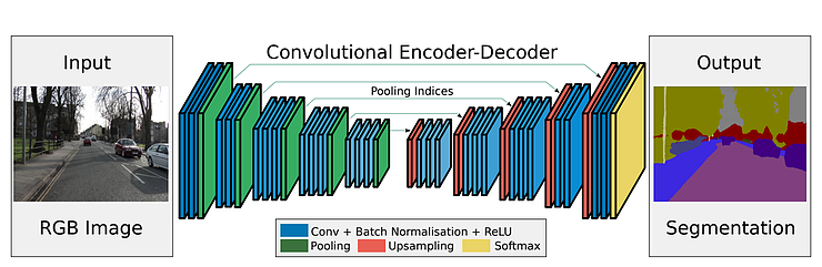
As shown on the above graph, SegNet is composed of a symmetry network: the encoder(left) and the decoder (right). The input is an RGB image and the output is a Segmentation image, where each color represents a semantic tag of objects. (e.g. “road”, “car”, “building” etc). Compare to SSD, which is an object detection network that does similar job (our previous post), SegNet gives out a more accurate 2D location of the object rather than a single bounding box. Moreover, road free space or road markings also can be obtained, which are extremely helpful in Autonomous Driving.

Encoder

Although the encoder has a fancy name, it is nothing special other than regular Convolution Neural Networks. It composes three types of network: Convoution, Pooling and Batch Normalization. The Convolution Layer extract local features, the Pooling Layer downsample the feature map and propagate spacial invariant feature to deeper layers and the Batch Normalization Layer normalizes the distribution of the training data aiming at accelerating learning.
Basically, the encoder extracts high-level information (such as “car”, “road”, “pedestrians”) from low-level image information, which are plain colored pixels. The decoder then receives this high-level information and map it into another medium level and reform it into an image with the same size, where objects with the label (such as “car”, “road”, “pedestrians”) are given the same color.

Another way of thinking Encoder+Decoder

Here is how I consider this process. Suppose you have a book of recipe and this book has many chapters, each chapter is written in English words to describe how to cook different dishes. Then we input all words of the book to the SegNet. Note that at this moment, SegNet does not know anything about the structure of the book. What the Encoder does is that it learns and understands the structure of the book, abstracts each chapter’s content and re-represents them in a simplified high level. The SegNet now knows what types of dishes the book teaches and is able to represent each chapter in a simplified form. The Decoder then reinterpret this high level information and label the words that are semantically similar. As a result, each word in the book is categorized and labeled. (For example: “Appetizer”, “Spaghetti”, “Fish”, “Steak”, “Pizza”, etc.). By only looking at some words, you will know that whether they are related to “Appetizer” or “Spaghetti” or something else. In other words, not only can you obtain the category but also you know what category a word in a page refers to. How great is it!

So if we go back to the example of an image, what the Encoder does is that it analyzes and figures out what and where the objects are, while the Decoder maps the objects back to the pixels that the label refers to. Boom! All pixels are segmented!

Pooling, Upsampling & Pooling Indices

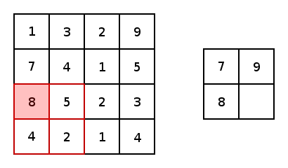
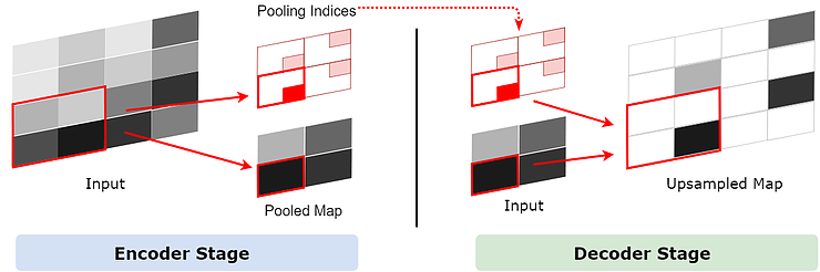
In SegNet, a non-overlapped 2×2 max pooling is adopted as illustrated below. Only the maximum value inside this 2×2 region is kept and propagated to the next layer.

Upsampling, is just the opposite way of pooling. However, there is one uncertain fact that during Upsampling, the size of 1×1 becomes 2×2, one of which will be taken by the original 1×1 feature and others will be empty. But which location should be assigned to the original 1×1 feature? We can assign it randomly or in a fixed way, but this might add errors to the next layer. The deeper it goes, the more it affects the layer that follows so it is important to keep the 1×1 feature in its proper place.
In SegNet, this is implemented through a so-called Pooling Indices. On the Encoder stage, the index of the maximum feature in each 2×2 area is saved for Decoder to use. Now that we have the Pooling Indices and given the fact that the whole network is symmetric, during Upsampling on the Decoder stage, the 1×1 feature goes to the exact location where the corresponding Pooling Index shows, as illustrated in the graph below.

Convolution Layer in Encoder and Decoder

The Convolution Layers exist in both Encoder Stage and Decode Stage. They work mechanically the same but have slightly different meanings. In Encoder Stage, the Convolution Layer extracts local features and pass them to Pooling Layers, which subsamples the input feature map by keeping the max value in the 2×2 area. You can think that the Convolution+Pooling in Encoder Stage learns to “extract” features.

On the contrary, in the Decoder Stage, the input feature map is first upsampled before going to Convolution Layers. In a 2×2 upsampled area, only one value is propagated from previous layer and others are empty. Later the empty spots will be filled up by Convolution Layer. So here, the Upsampling+Convolution learns to “add” features to the feature map in order to make it smother.

In a word, the computation behind these Convolution Layers are totally the same, but they somehow results in a impression that they behave differently. Some people name them after “Convolution” in the Encoder Stage and “Deconvolution” or “Transposed Convolution” in the Decoder Stage, but in fact the computation of these two make no difference. Here are two animations of “Convolution” (left) and so-called “Deconvolution”(right).

Our Implementation Model

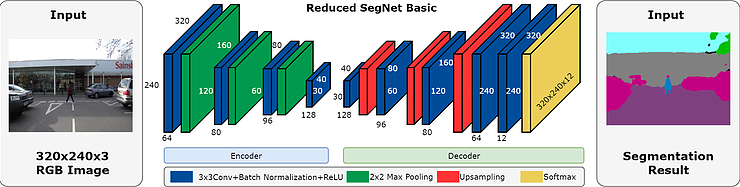
As the original SegNet model is a bit heavy for running on FPGA, we use an alternative model SegNet Basic and reduced some channels to improve the performance. The network architecture is shown below.

Demo GIF

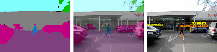
Here are some more results. You can see trees/buildings/cars/pedestrians are pretty well segmented.

SSD detection is also included for the purpose of comparison. The result shows that our AI accelerator DV700 is able to handle multiple network running at the same time! This is exciting because in real-world autonomous driving applications, tasks involving different networks may need to be running at the same time.

(The SSD used in this experiment is trained for traffic scene with a small dataset and is still under development so that you may find some false detection.)

Reference

• SegNet Paper
• Pooling Animation
• Convolution Animation
• Deconvolution