This post demonstrates the Single Shot Multibox Detector(SSD) result on PC and FPGA. We will go over the key features of SSD and hope you can grasp the big picture of SSD after reading this post.
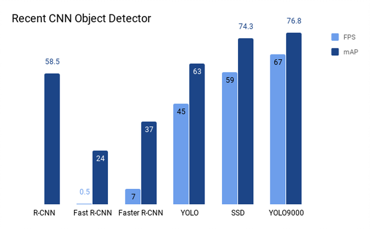
Convolutional-Neural-Network Based Detector has made great improvement over the years, making it possible to perform classification and localization at the same time. But there used to be a bottleneck in computational cost until YOLO was introduced. It achieved hundreds times of speed improvement compared to previous work while keeping a high mean Average Precision (mAP). SSD then achieved better results in both FPS and mAP. Although later YOLO 9000 proved even better results, SSD is definitely an outstanding work to study.
SSD demo on PC
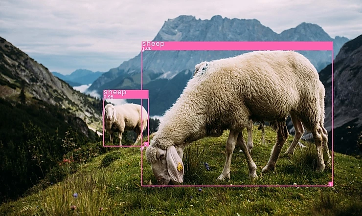
Let’s see the demo first! We used a tensorflow implementation of SSD in this demo. There are 20 classes trained on Pascal VOC 2007+2012 dataset. The input video shown in the demo can be found here. Also, classes that do not show in the video are also tested with images selected from unsplash.com. The SSD detection module runs about 20 FPS @i7-7700 CPU 3.6GHz and NVidia 1050Ti GPU.
SSD demo on FPGA
Although SSD can almost run on PC at real-time, it is still computationally expensive for mobile devices or embedded-systems, as most object detection target system are not PC-based.
Here is another SSD real-time (19.8FPS) demo running on FPGA board (ZYNC ZC706)@70MHz. The CNN accelerator DV500/DV700 used in this demo is developed by one of our team member and supports most Deeplearning Framework including Keras, Caffe etc.
Single Shot Multibox Detector Overview
By taking a look at the graph below, you may start having questions such as: What makes SSD different from others? Why does SSD improve greatly on FPS? We will go over the key features of SSD by answering these questions. If you are interested in thorough understanding of SSD, here is a nice post recommended.
Let’s first have a look at the flow diagram of SSD then we will briefly explain each key feature that makes SSD different.
What makes it fast?
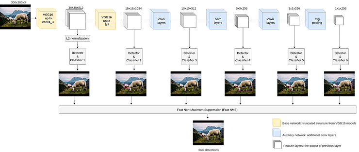
The SSD Network Structure – A single feed-forward deep Neural Network.
SSD takes an image as an input and directly outputs the bounding box (bbox) and classification confidence, which, in R-CNN generations, is done through multiple phases that are computational expensive. (E.g. Training the region proposal and classifier separately)
What improves the accuracy?
As can be seen from the flow diagram above, the sizes of feature layers decrease gradually and when new feature layers are generated by previous conv layers, detection and classification are carried out on every of them. Then the detection results are merged during Fast NMS process to generate the final detection result. This structure helps the network detect multiple-scale objects. As convolution layer only “sees” local information, the deeper it goes, the bigger object it can see. This makes sure that objects of different scales (or sizes) can be detected, thereby improving the accuracy.
How does SSD make bbox proposals?
Unlike R-CNN, which first propose a number of object candidates and then compute how likely this candidate belongs to a certain class, SSD has a fixed number of default bboxes in each feature layer. Each cell in the feature layer represents a group of default bboxes in different locations, scales and aspect ratios. In detection, the confidence of which a bbox belongs to a class is computed. The total number of bboxes per class used in the paper is 7308. Only top N bboxes with confidence greater than a threshold (i.e. 0.5) are passed to Fast NMS, where redundant bboxes are removed and the final detection bboxes are kept.