Introduction
YOLOv3 is the third object detection algorithm in YOLO (You Only Look Once) family. It improved the accuracy with many tricks and is more capable of detecting small objects. Let’s take a closer look at the improvements.
The algorithm
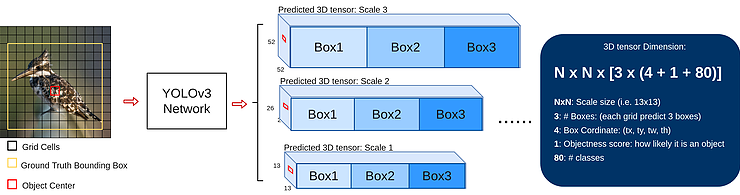
First, during training, YOLOv3 network is fed with input images to predict 3D tensors (which is the last feature map) corresponding to 3 scales, as shown in the middle one in the above diagram. The three scales are designed for detecting objects with various sizes. Here we take the scale 13×13 as an example. For this scale, the input image is divided into 13×13 grid cells, each grid cell corresponds to a 1x1x255 voxel inside a 3D tensor. Here, 255 comes from (3x(4+1+80)). Values in a 3D tensor such as bounding box coordinate, objectness score and class confidence are shown on the right of the diagram.
Second, if the center of the object’s ground truth bounding box falls in a certain grid cell(i.e. the red one on the bird image), this grid cell is responsible for predicting the object’s bounding box. The corresponding objectness score is “1” for this grid cell and “0” for others. For each grid cell, it is assigned with 3 prior boxes of different sizes. What it learns during training is to choose the right box and calculate precise offset/coordinate. But how does the grid cell know which box to choose? There is a rule that it only chooses the box that overlaps ground truth bounding box most.
Lastly, how to choose the initial size of those 3 prior boxes? The author uses K-mean clustering to classify the total bboxes from COCO dataset to 9 clusters before training. This results in 9 sizes chosen from 9 cluster, 3 for 3 scales. This prior information is helpful for the network to learn to compute box offset/coordinate precisely because intuitively, bad choice of box size make it harder and longer for the network to learn.
The Network Architecture
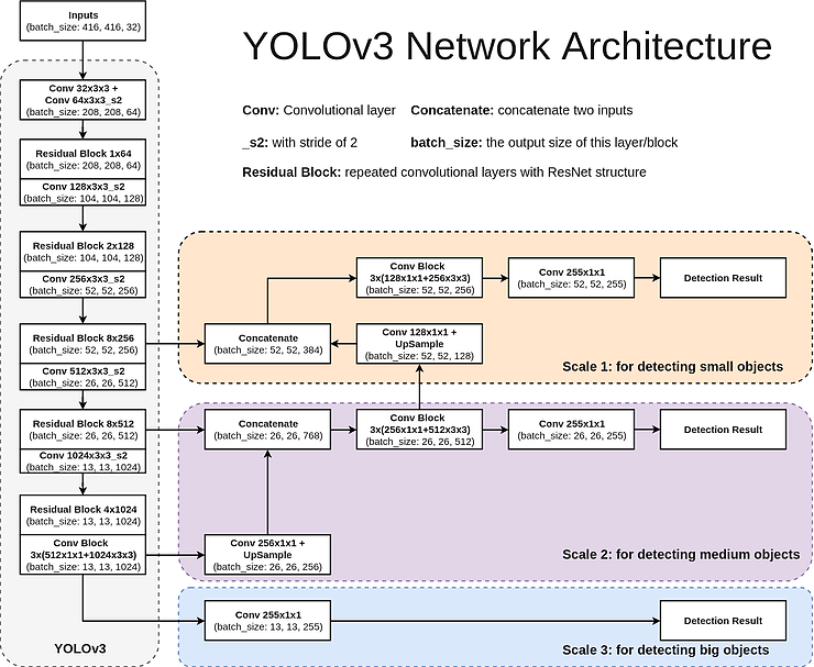
Here is a diagram of YOLOv3’s network architecture. It is a feature-learning based network that adopts 75 convolutional layers as its most powerful tool. No fully-connected layer is used. This structure makes it possible to deal with images with any sizes. Also, no pooling layers are used. Instead, a convolutional layer with stride 2 is used to downsample the feature map, passing size-invariant feature forwardly. In addition, a ResNet-alike structure and FPN-alike structure is also a key to its accuracy improvement.
3 Scales: handling objects of different sizes
There are objects of different sizes on the images. Some are big and some are small. It is desirable for the network to detect all of them. Therefore, the network needs to be capable of “seeing” objects that are of different sizes. As the network goes deeper, its feature map gets smaller. That is to say, the deeper it goes, the harder it is to detect smaller objects. Intuitively, it is better to detect the objects at different feature maps before small objects end up disappearing. As in SSD, object detection is carried out on different features maps in order catch various scales. (see our previous post about SSD)
However, the features are not absolutely relevant at different depth. What does this mean? Well, with network depth increasing, the features change from low-level features (edges, colors, rough 2D positions. etc) to high-level features (semantic-meaningful information: dog, cat, car. etc) with depth increasing. So making predictions on feature maps at different depth does sound it is able to do detection for multi-scale objects, but actually it is not as accurate as expected.
In YOLOv3, this is improved by adopting an FPN-like structure.
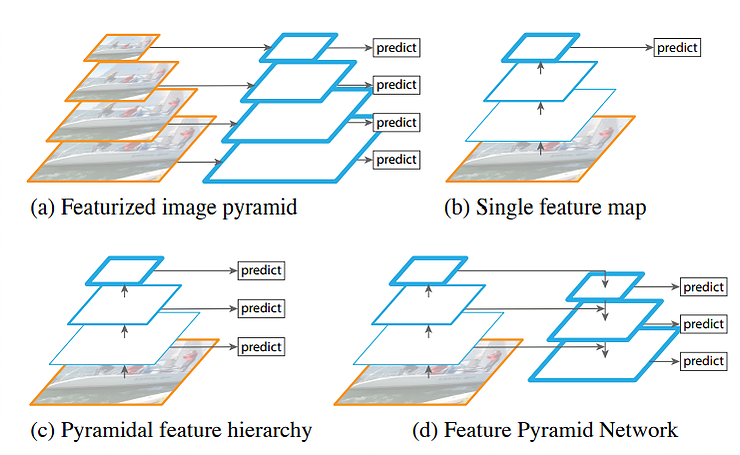
As shown on the above illustration, there are 4 basic structure for multi-scale feature learning.
(a) The most straightforward one. Construct an image pyramid and input each pyramid level to individual network specially designed for its scale. As a result, it is slow because each level needs its own network or process.
(b) The prediction is done at the end of the feature map. This structure cannot handle multiple scales.
(c) The prediction is done on feature maps at different depth. This is adopted by SSD. The prediction is done by using the features learned so far and further features at deeper layers cannot be utilized.
(d) Similar to (c) but further features are utilized by upsampling the feature map and merged with current feature map. This is fascinating because it let current feature map to see its features in “future” layers and utilize both to do accurate prediction. With this technique, the network is more capable to capture the object’s information, both low-level and high-level.
ResNet-alike structure: a better way to grasp good features
In YOLOv3, a ResNet-alike structure (called Residual Blocks in the YOLOv3 Architecture Diagram) is used for feature learning. Basically a Residual Block consists of several convolutional layers and shortcut paths. An example of a shortcut path is illustrated below.
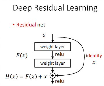
The curved arrow on the right represents a shortcut path. Without this, it is a classic CNN network, which learns the feature one by another. As the network goes deeper, the harder it is to learn the features well. If we add a shortcut as shown above, the layers inside the shortcut learns what to add to the old feature in order to generate better feature. As a result, a complex feature H(x), which used to be generated standalone, is now modeled as H(x)=F(x)+x, where x is the old feature coming from the shortcut and F(x) is the “supplement” or the “residual” to learn now. This makes it easier for the network to learn the features stably, especially in very deep networks. This technique changes the goal of learning. Thus, instead of learning a complete complex feature, the new goal is to learn the supplemental “residual” that is used to be added up to the old feature, which simplified complexity for learning.
No softmax layer: multi-label classification
Softmax layer is replaced by 1×1 convolutional layer with logistic function. By using a softmax, we have to assume that each output only belong to exactly ONE of the classes. But in some dataset or cases where the labels are semantically similar (i.e. Woman and Person), training with softmax might not let the network generalize the data distribution well. Instead, a logistic function is used to cope with multi-label classification.
Demo GIFs
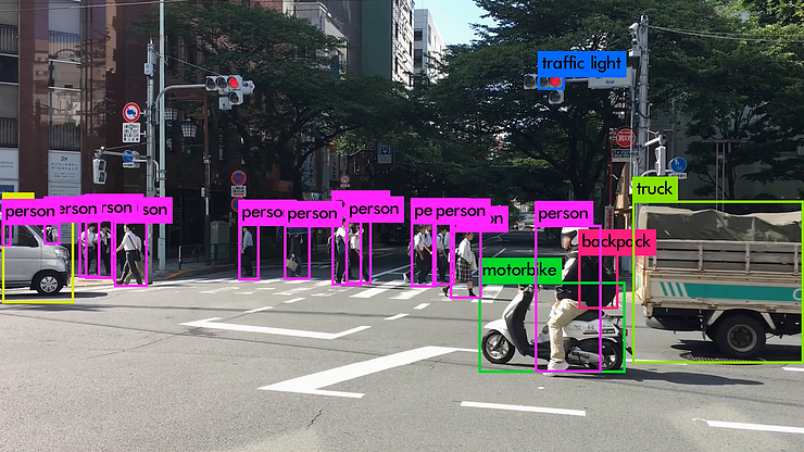
Here are some demo clips shot on different scenes and objects. It does pretty well in small object detection. Also, close objects such as “A person riding a bicycle/motorcycle” can be detected separately. Besides, densely grouped objects can also be detected.
YOLOv3 Performance on Desktop PC
– Official: 29ms @Titan X GPU
– Ours: 76ms @1050Ti GPU
Tiny YOLOv3
YOLOv3 indeed is more accuracy compared to YOLOv2, but it is slower. Fortunately, the author released a lite version: Tiny YOLOv3, which uses a lighter model with less layers. With this model, it is able to run at real time on FPGA with our DV500/DV700 AI accelerator. Here is a real-time demo of Tiny YOLOv3.
Tiny YOLOv3 Performance on FPGA
- Platform: FPGA+DV500/DV700 AI accelerator
- Board: ZYNC ZC706
- Performance: 30 millisecond / frame
*Since the video is captured by a live USB camera, there are some drops in latency and image quality, which affects the detection accuracy a bit.
Reference:
- YOLOv3 Tech Report: This report is fun to read.
- YOLOv3 Implementation: Easy to try. Just follow the instructions.
- Feature Pyramid Networks for Object Detection: The paper
- Deep Residual Learning: The presentation slides